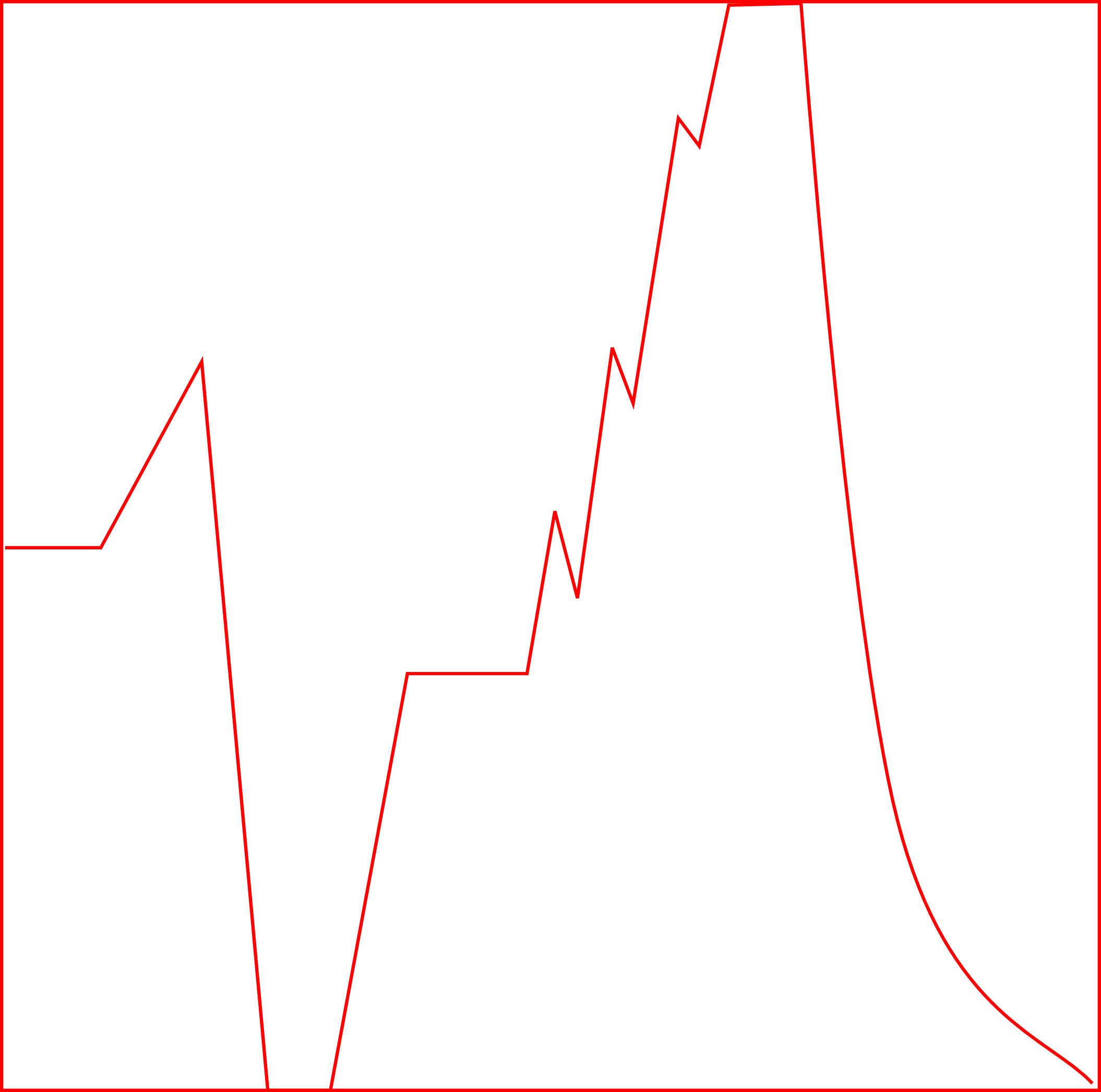
Shape used as the basis for Shape06
Lou Cohen - Method of Composition
Lou Cohen uses Csound as his primary tool for realizing compositions.
Csound is a well-known, open-source, programmable music synthesizer.
Its antecedents (called "MUSIC", "MUSIC II", "MUSIC III", ... )
were developed by Max Mathews
at ATT Bell Labs starting in the 1950s.
"MUSIC 11" was written by
Barry Vercoe at the MIT Media Lab.
Vercoe then rewrote this software and renamed it as Csound. Eventually Csound
was given open-source status, making it freely available.
Csound has gone through many versions since then, has a team of
volunteer developers, has thousands of users around the world, and
runs on many different computer platforms. For more about Csound,
visit the official Csound website.
With Csound as an underlying tool, Cohen employs three methods for most
of the compositions on www.jolc.net. These methods correspond to this
grouping of the compositions:
1. Method for "shape" compositions and "harmonies"
For the "shape" compositions and "harmonies", the first step is to draw a geometrical "curve" or "shape," such as:
Shape used as the basis for Shape06
Using an open-source utility program, this shape is then digitized, so that it can be represented by a series of number-pairs, representing x- and y- coordinates corresponding to the shape.
The horizontal axis of the shape represents time, both a very short amount of time for some aspects of the composition, or a rather long time for other aspects of the composition. The vertical axis is variously used to represent many aspects of the music, as described in the next few paragraphs.
First, the shape is used to represent the wave-form that will be rendered by Csound to create all sounds. As a wave-form, the shape would be cycled scores, hundreds or thousands of times per second, thus having a frequency in the 20 Hz to 3000 Hz range.
Second, the shape (or its inverse, retrograde or retrograde-inverse) is used as a control signal, cycling once or a few times over the length of the entire composition, thus having a frequency in the 0.001 Hz to 0.01 Hz range.
As a control signal the shape is used to determine all aspects of the playing of notes: density of notes (number of notes played per second; that is, the onset rate), frequency (pitch) of each note, duration of each note, amplitude of each note, rise and decay time of the amplitude envelope of each note, and other aspects of the sound of each note, such as rate and intensity of any vibrato. In some of the "shape" pieces "ornaments" occur. These "ornaments" consist of short rapid sequences of notes selected by a computer algorithm to be relatively close to an already determined note. Various characteristics of these ornaments are also determined by the control signals.
The algorithms for interpreting and using the control signals as well as the wave-form are written in Csound code.
Typically three or four tracks are created for a composition, where each track uses the control signals in somewhat different ways. The tracks are then mixed together for the final composition.
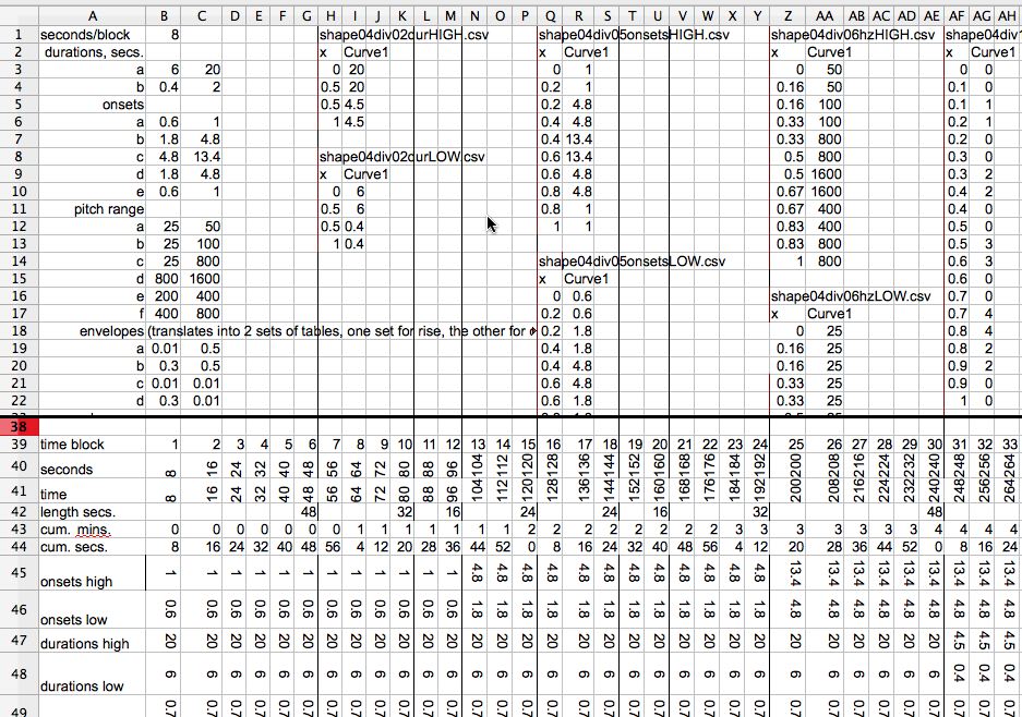
Screen shot of portion of the spreadsheet used for planning
"shape04." Upper portion shows numeric definitions of various shapes
used in the composition. Lower portion outlines the succession of
sections in the composition, showing parameters controlling density
(offsets), frequency, duration, etc.
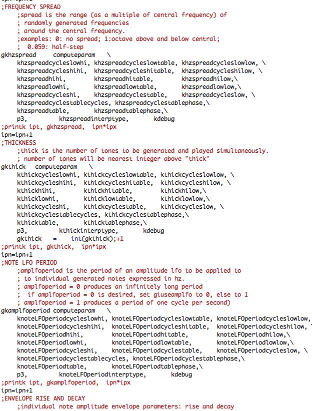
Screenshot showing a portion of the Csound code used for
"shape04." This section shows code that converts the "shapes" into
control signals that will be used to generate bursts of sound. This
code is executed 4,410 times for each second of generated sound.
2. Method for "Circles"
"Circles" uses several instances of a single "shape," the circle. The circles are represented by equations which describe these circles in a multi-dimensional space. The various dimensions in space correspond, as with the "shape" compositions, to the density of notes, as well as duration, amplitude envelope, pitch, amplitude, and other aspects of each note.
As the path of a circle is traversed over time, the circle is traversed through space. Therefore these characteristics vary, hence the sound of the music varies. The path, in time, of each circle through space results in a track of sound. The equations have been set up in such a way that the circles travel through the sound-space on different paths, but are designed to come in contact with each other somewhere (and at some time) during the composition. The effect is that the sounds of the tracks are identical when the circles are in contact, but then diverge as the paths of the circles diverge. The sounds then converge again as the paths of the circles once again approach the contact points.
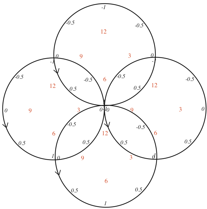
One of several diagrams drawn by the composer for the
production of "Circles." The red numbers are simply clock-hours for
easy reference to positions along the circle. The black numbers represent
values taken on by the mathematical function sin(t), as the variable "t"
moves through time. The circles in this diagram are being traversed
counter-clockwise, as indicated by the arrow heads. The intersections
of the circles are linked to important moments in the final composition.
3. Method for "Symphonies"
The Symphonies all share yet another technique. In this case, a selection of sound samples is assembled. These samples could be of acoustic instruments, such as violins, drums or clarinets; or they could be samples of synthetic sounds. In either case, the samples are installed in a soft-sampler and played back by the composer improvising at a MIDI keyboard. This results in one or several audio "source" files containing the results of these improvisations.
Then a series of Csound commands are generated by means of a computer program written by the composer (see screenshot below.) This program accepts a wide range of data parameters and generates thousands or tens of thousands of Csound commands. The commands instruct Csound to copy thousands of minute snippets of sound from the source files, and paste these into a final composition.
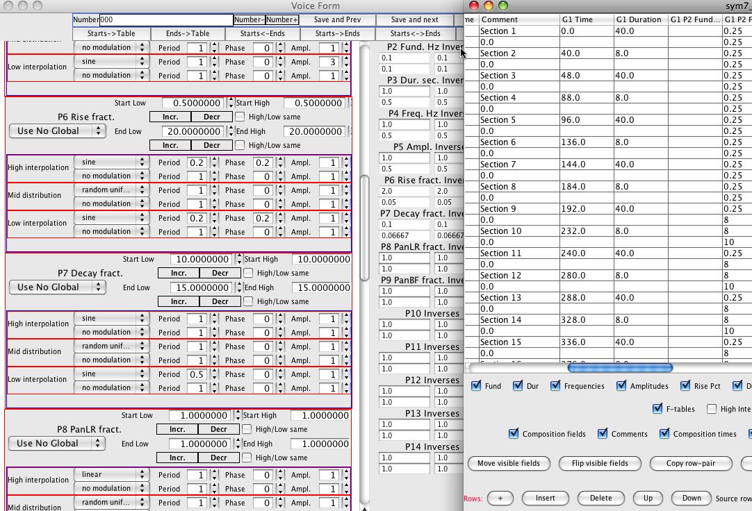
Screen shot of the main windows of "Gestures," a
computer program written by Lou Cohen. This particular screen
shot is for "Symphony 7."
The left-hand window is used for setting parameters for a single
"gesture." A "gesture" is a segment of sound, typically 5 to 30
seconds. During that period of time, many Csound commands representing
short bursts of sound will be generated by "Gestures." The characteristics
of those bursts are displayed and controlled in the left-hand window.
The parameters shown in that window determine the density of bursts
(how many bursts per second), the duration of each burst, the waveform
of the bursts, the frequency of the waveform for each burst, the amplitude
of the bursts, amplitude envelope of the bursts, and additional parameters
that could be used by Csound to further tailor the bursts of sound.
Each parameter (density, duration, etc.) may evolve in time over the
duration of the "gesture." The nature of these evolutions (increase,
decrease, follow a sinusoidal path, vary randomly, ...) is specified
in the left-hand window.
The right-hand window displays all the "gestures," in the composition.
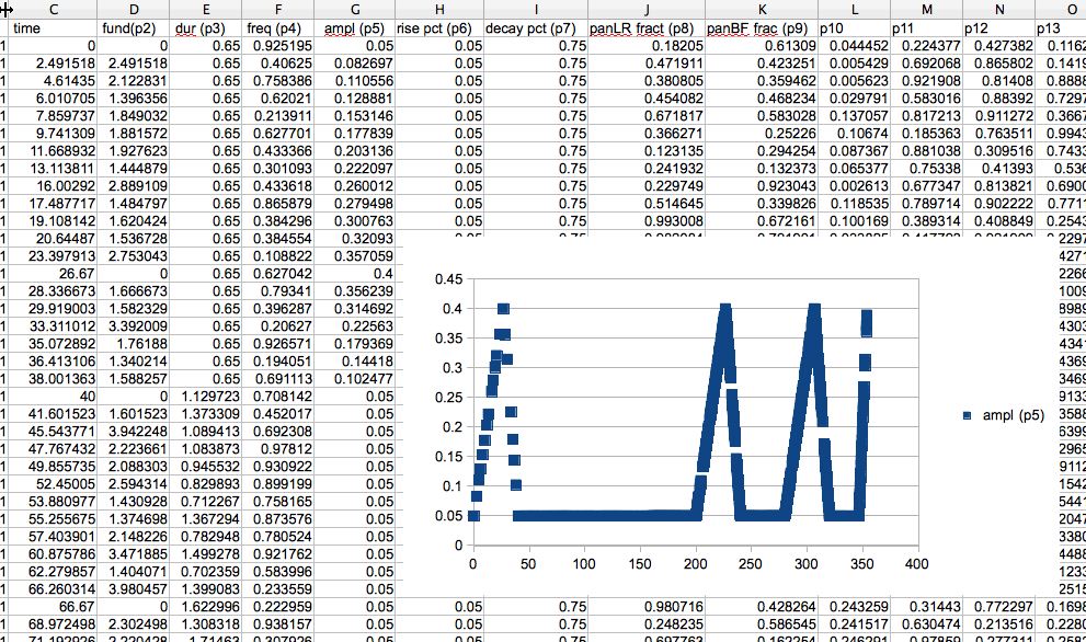
Screenshot of a spreadsheet displaying "Gestures"
output for "Symphony 7." Time in seconds is displayed in column
C; parameter headings are across the top of the spreadsheet.
The graph shows the values for amplitude bursts over time.
Amplitude is in the scale of 0 to 1. The x-axis displays time
in seconds.
4. Orthogonal Arrays
Orthogonal Arrays (OA) were first described by the great mathematician Leonhard Euler (he called them "Orthogonal Latin Squares".) These were generalized by Dr. Calyampudi Radhakrishna Rao and made known to Cohen by the work of Dr. Madhav Phadke, Dr. Don Clausing and Dr. Genichi Taguchi. Their application of the OA was aimed at increased quality and reliability of manufactured products, such as automobiles. However, the OA concept has been used in a wide variety of applications since Taguchi's early work, including software testing design, and as described here, in the process of composing music. Cohen uses OAs to select manageable numbers of diverse combinations from very large universes of combinatorial possibilities.
OAs provide a subset of all possible combinations of any factors with certain key symmetries present. An example will illustrate the ingenious design of the OA. Let us say we want to write a piece for five timbres, which we shall call t1, t2, t3, t4 and t5. Further, we want to maximize timbral variety by using these timbres in many different combinations. In the parlance of OAs, the timbres will be called "factors." We further decide that each timbre could be heard with any of three amplitude envelopes, which we shall call e1, e2 and e3. In OA parlance these different possible assignments envelopes to timbres are called "levels." To start with we might consider all combinations of factors at all possible levels, that is, the "full factorial" set. However, the full factorial set consists of 3 to the 5th power of combinations: that is, 243 combinations. This is an exhaustive list of all possibilities of 5 timbres (t1, t2, t3, t4 and t5) played at each of 3 envelopes (e1, e2 and e3.) 243 combinations are too many to work with. To use them all would make a composition too long. We could select only some from this long list, but how to ensure a diverse collection of possibilities? One must select judiciously from the entire list to achieve maximum variety with a manageable number of selections. The Orthogonal Array provides an excellent way to guide the selection process.
Hundreds of basic OAs are readily
available at websites (for example: http://www2.research.att.com/~njas/oadir/)
and in books that list them. For our example, we need to find one that fits our
particular problem.
Since we have 5 timbres (factors), the orthogonal array must have at least 5 columns -
each corresponding to one of the timbres. Each timbre can be played with
amplitude envelope e1, e2 or e3, so we need an
Orthogonal Array with at least 5 factors (columns) and three "levels"
(3 different numerical values in the cells of the arrays.) By consulting a
book of orthogonal arrays, we find that the Orthogonal Array called "L18" has
8 factors (columns.) Column 1 has 2 levels (1 and 2), and columns 2-8 each have
3 levels (1, 2, 3). We are not required to use all the columns: we can use
only as many as we need for our problem.
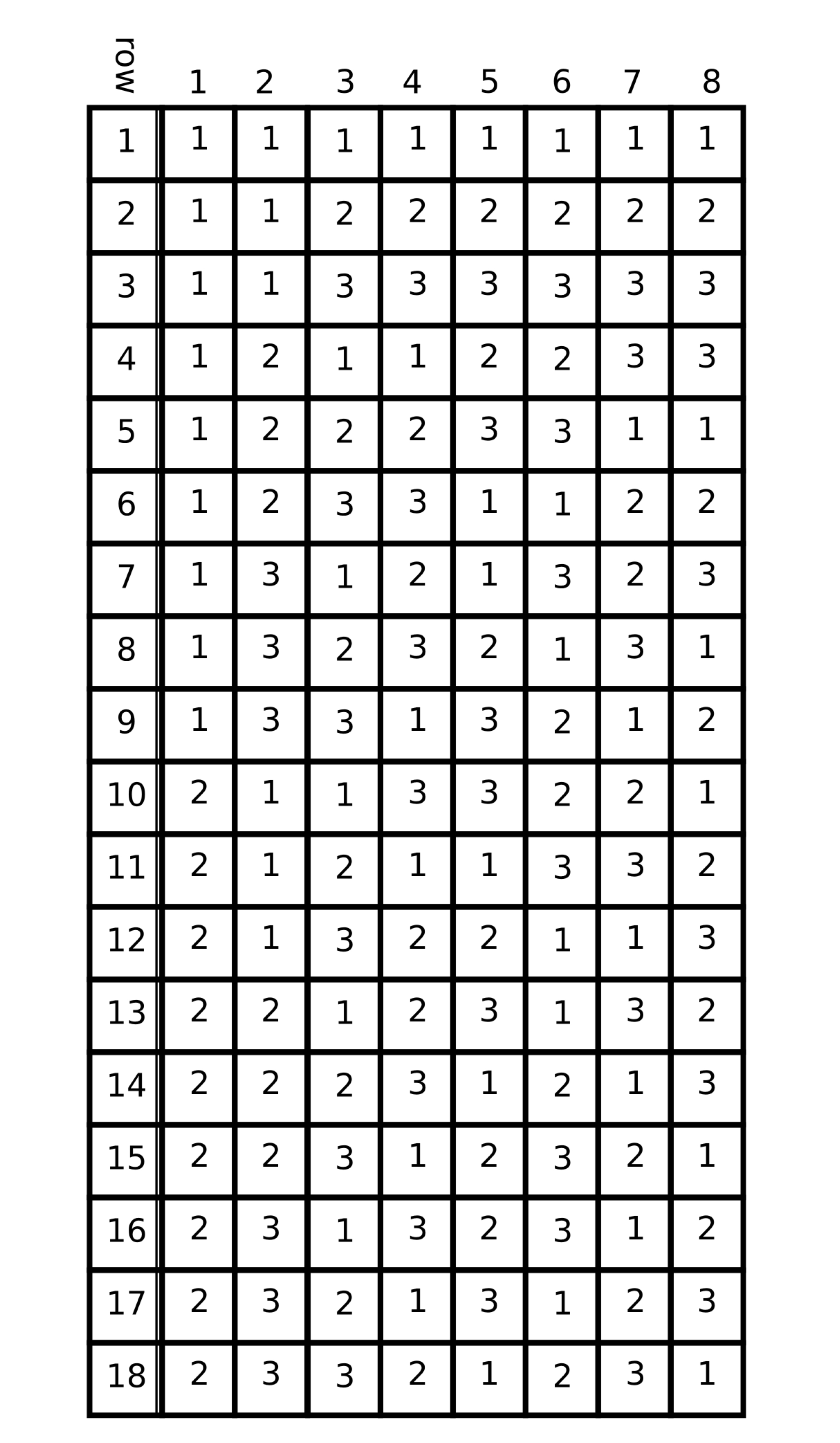
Orthogonal Array "L18."
Of all the many OAs, L18 is widely used
because it has a reasonable number of factors and levels and it's quite small
(only 18 rows.) Each of the rows in the OA represents one selected combination
of the factors at various levels. To apply L18 to our problem, we will use
18 combinations, corresponding to rows 1-18. We require 5 columns, corresponding
to timbres t1, t2, t3, t4 and t5, so will make these assignments:
Further, we can use the numbers in the cells of the array to assign amplitude envelopes to each occurrence of each timbre. For example, reading cells in row 11:
If we decide that envelope 3 results in silence, thus muting its associated timbre, then the assignments for Row 11 become: